This blog explores the basic ideas of Consumer Theory, like Indifference Curves, Utility functions, etc., in a beginner-centric approach.
Consumer Theory deals with how consumers decide to spend their money given their preferences and budget constraints. It can be also referred to as a set of assumptions about human nature, and how they arrive at a decision to purchase a particular set of items, in a sea of options.
Utility Functions
Introduction
Utility can be described as the ‘usefulness’ of a particular set of item(s). To give you a better grasp, think of it as the customer satisfaction when he/she buys a particular set of item(s). Confusing right?, Before you get any new ideas, I would like to point out that most of Consumer Theory is simple, everyday human interactions boiled down to simple math using varied assumptions. So, in between if you feel confused, don’t worry, just go back to the assumptions and start again :)
Now coming back to Utilities, we described Utility to be the ‘usefulness’ of a particular combination of item(s). The function which calculates the Utility of a set of item(s) by taking some inputs (i.e. the individual quantities) is known as the Utility Function. For example, if U is the utility and A and B are the quantities of apples and bananas. Then,
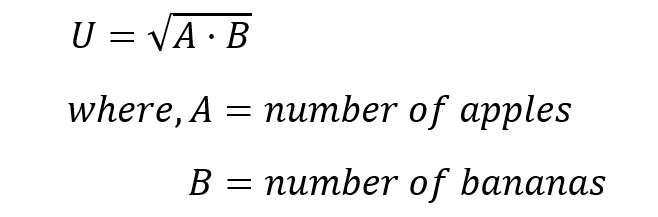
Makes sense? :)…I hope not.
Most utility functions are of this form (this is too simple)….why? well you’ll see :)
Now lets continue on with our assumed Utility function.
‘More the Utility, happier are you’.
Assumptions
Remember, I told you there are a lot of assumptions to be made. Let’s start off :)
- Completeness — You are complete and rigid in your decisions. If you prefer 10 apples today over bananas, then you will prefer the same tomorrow as well provided the constraints remain the same. Simple right :) ?
- Transitivity — If you prefer apples over bananas and bananas over melons, then you prefer apples over melons as well :)
- Non-Satiation — ‘More is always better’. You always prefer more stuff compared to less, more Utility than less, more number of apples than less.
Done for the day, these were the ‘sick’ assumptions whose only purpose is to make our math and logic simple.
Indifference Curves
This is where things get interesting. Let’s start with our ‘great’ utility function —
Think about this —
Set 1 — You have 10 bananas and 20 apples.
Set 2 — You have 20 bananas and 10 apples.
I give you the liberty to choose any set. Which one will you choose?
Well, you can’t, right!..Cause the Utility value for both these cases is same i.e sqrt(200). Remember you only choose higher Utility over lower.
That’s what an Indifference Curve is: It is a graphical representation of different combinations of A and B, which yield the same Utility value and hence, you are indifferent towards them.
‘People always prefer higher ICs’.
 |
|---|
| ICs are always convex to the origin. |
Marginal Utility
Let us comeback to our original Utility function —
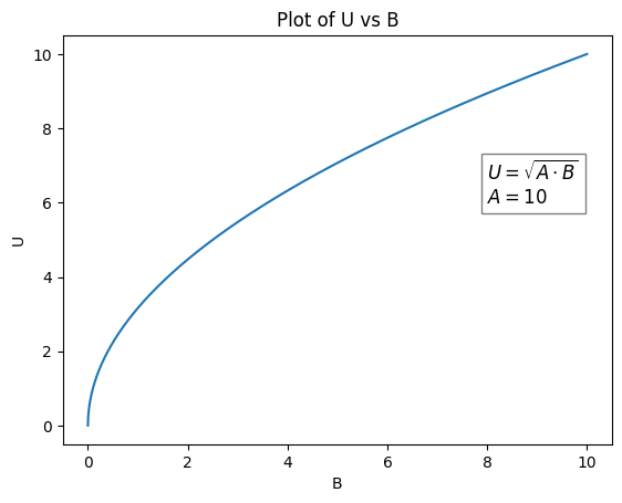
And plot Utility function U with respect to B, while keeping A constant. It looks something like this —
 |
|---|
| Marginal Utility decreases as B increases. |
Look at the curve above closely. Do you see something strange….
Or maybe try looking at how U changes depending on B.
If you weren’t able to make it out, let me make it out for you —
Observe that when B is large, a change in B produces a small change in U. And similarly, when B is small, a change in B produces a large change in U. Change in Utility decreases as B increases.

 |
|---|
| The rate of change of U with respect to B decreases. |
The more bananas you have, the less the change in Utility (Usefulness).
It’s as if ‘that extra banana(B) does you no(less) good.’ Or, in other words — ‘the more you have something, the less you want it.’
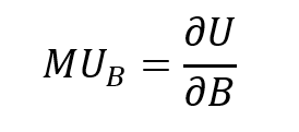
Mathematically, you can say it is the rate of change of U with respect to B:
 |
|---|
| Marginal Utility of B |
Marginal Rate of Substitution
If you were able to grab the whole meaning of the above topic, the rest is just a piece of cake.
Let us again come back to our Indifference Curve (IC) — observe the slope while moving from point P1 to point P2. Let us say it as S1. Similarly, for points P2 to P3, S2.

Noticeably, S1 is quite greater than S2. What does that mean?
Let us look the path 1 (points P1 to P2). We move 5 steps in the x-direction and go down 20 steps in the y-direction. It’s equivalent to saying — we lost 20 apples (y-direction) to gain 5 bananas (x-direction). And that’s just for path 1, i.e. points P1 to P2.
Now let’s look at points P2 and P3. Interestingly, here you are only losing 10 apples while gaining 20 bananas. Numbers are quite the reverse of the first case. What’s happening here? why is the value of bananas in terms of apples varying?
Well, to answer that, let us again examine path 1 i.e., points P1 to P2. To reiterate it again, we lost 20 apples while only gaining 5 bananas. Therefore, the exchange set the value of each banana as 4 apples. You give 4 apples and get 1 banana. The reason behind this is simple — at point P1, you have more apples and fewer bananas. Hence, bananas became more valuable. Or in other words, you are willing to give up more apples to gain bananas.
Similarly, for points P2 to P3, you always have more bananas than apples, which automatically sets apples more valuable. Hence, you’ll be willing to exchange more bananas for each apple.
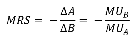
Mathematically you can define it as the slope of the line joining any 2 points on the Indifference Curve. And can be equated as:
Budget Constraints
Budget
Much of our discussion until now has been mostly about quantities and utilities and hasn’t really focused on topics like prices and budget, which arguably are one of the most important factors driving consumer behavior.
Before opening up the discussion, I would like to state an assumption:
- Your income is your budget — Assume that your budget while buying a set of products is always the same as your income, i.e., you have zero savings and money for other purposes.
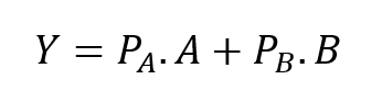
Now let’s start: Assume you have a budget/income of $Y. The price of each banana is $Pb, and each apple is $Pa. As we know from previous discussions, A is the number of apples, and B is the number of bananas. Combining these inputs — we get the formula:
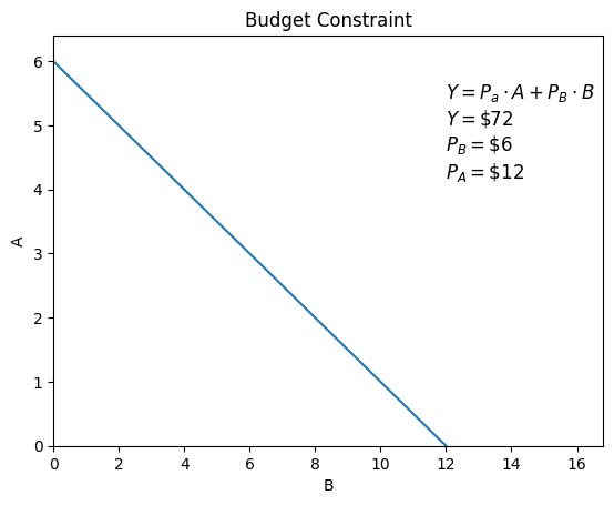
Plotting this equation on a graph gives the form:
Marginal Rate of Transformation
Think of it as similar to the Marginal Rate of Substitution, but rather than dealing with individual quantities, you deal with individual prices.
From the budget constraint plot, we can make out that for each banana is worth = slope * each apple.
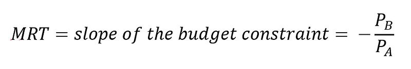
Hence, looking at the above plot, one can deduce that the Marginal Rate of Transformation = slope of the budget constraint line.
Income and Price Shifts
Now that we are quite done with the budget constraint and ICs let us look at what happens when we ‘shock’ the budget constraint, i.e., change the individual prices.
Imagine you have the same setup as before:
Y = Income/Budget
Pa = Price of each apple
Pb = Price of each banana
A = Quantity of apples.
B = Quantity of bananas.
and the corresponding budget constraint plot:
Case 1: Price of apple increases.

As you can see the y-intercept of the plot goes down implying that you’ll be able to buy only fewer apples even in your full budget. Also, with it the Marginal Rate of Transformation (MRT) has decreased as well. What does it imply? think!
Case 2: Price of bananas increases.

The x-intercept of the plot decreases, implying a decrease in your ability to buy bananas now. Also, interestingly, the MRT increases. Why?
Case 3: Budget increases.

Here as you can see, the slope (MRT) remains the same while the x-intercepts and y-intercepts increase, implying an increase in your ability to buy both products in increased quantities. The ‘level’ of the curve increases.
In general, the prices Pa and Pb are set by the market and hence cannot be controlled individually. Hence, it is said, ‘You can control the level, but not the slope’.
Constrained Choice
If you are reading till this far, congrats cause this will be the last topic for this blog.
Remember, before; we talked about different combinations of bananas and apples and how some combinations are ‘indifferent’ to us as they give the same utility value. In this part, we’ll tackle the problem of choosing a combination when your Utility function and budget constraints are well defined.
Remember — If your budget constraint weren’t defined, then you would go for the maximum number of apples and bananas as they would maximize the Utility function.

To answer this question — we can look at the combined plots and, thereby, arrive at our answer.
In the above plot, we plotted different IC curves (different U values) and the budget constraint (red). Now the question is — which indifference curve and, more importantly, which combination would give me maximum Utility while being within the budget constraint?
Plot A (Blue): This IC crosses the budget constraint twice, i.e., there are 2 points in the IC that satisfy the budget constraint. But the Utility values for this IC are the smallest among the 3 (most inward IC). So, reject it.
Plot C (Green): This IC does not cross/touch the budget constraint at any point. Even if it has the largest Utility value, it is useless because combinations of this IC do not fall under our budget constraint. Therefore, rejected.
Plot B (Orange): This IC just touches our budget constraint and gives us the largest value of Utility while also being in the budget constraint. Hence, it is the most optimal IC, and the point, i.e., (6,3) touches the budget constraint, is the Optimal Constrained Choice.
Fundamental Equation of Economics
Wait, hold up…I know I said it was the last topic, but just bear with me for one more topic — and probably the most important one.
In the above topic, we were able to find the Optimal Constrained Choice using the ICs of the Utility function and the budget constraint, as a point. But what is so special about this point? Think…..
Well, let me answer this for you — At this point, the Marginal Rate of Substitution equals the Marginal Rate of Transformation.

Mind-blowing right?
Phew, finally, we’ve come a full circle and connected both the basic ideas (ICs, Utility functions) and the theory of constrained choice (budgets, prices).
If you read this far, pat on your back, for you deserve a break.
We’ll end this blog here for now; there are a few more topics of interest (Demand Curve, Income Shifts) that are quite worthy of discussion and hence will discuss in the second part of this ‘series.’
Thank You…