
In this short blog, I’ll talk about the Costs of Production and how producers want to maximize production,and also some other topics as Isoquants, Sunk Costs etc.
In my last blog (link), I talked about production functions, Isoquants, and their behaviors in both the long-run and short-run time frames.
In this blog, I’ll discuss production costs and how firms choose what quantity of the product to produce. Let’s begin.
Cost of Production
Every firm needs to produce and sell goods to make money, but one cannot increase production indefinitely in hopes of increasing profits. There can be two reasons for that —
- There is only a limited demand for the product. Therefore, after a certain production level, the product does not sell.
- The cost of producing the product after a certain production level is more than what it is being sold for i.e. Firm is making a loss.
The first point is undoubtedly well-understood and intuitive. But the second point is the one that makes most of the difference for any firm.
For every product the firm produces, there is an inherent cost attached to it, be it their labor charges, rental rate of the offices, or machinery expenditure. And as you can guess, their value changes with the level at which they are producing. Therefore, based on the previous blog, their Cost Function(C) depends on the Production Level(q).
 |
|---|
| Cost is a function of q. |
Now to derive an expression for the above, let us first describe the Cost Function.
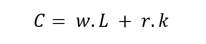
We know the cost depends on many things, but for the sake of simplicity, we will assume only two variables i.e. Labour(L) and Capital invested(k)
 |
|---|
| Cost function |
Where,
w = wage rate of the Laborers employed (L)
k = rental rate of the capital invested in machinery, space, etc. (k)
I hope it makes sense….
Now, let us divide this into different time frames: Short-Term and Long-Term.
Short Term
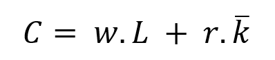
In the short term, we know Capital invested(k) is assumed to be constant, and from our previous discussions, we know:
 |
|---|
| Short-Run production function |
Then, Cost Function will become —
 |
|---|
| Cost function for short-term production |
Now, combining the above two equations together, we get —
 |
|---|
| Short-run production in terms of production level (q) |
Let us assume —
k_bar = $1
w = $5
r = $10
We get the equation modified as —
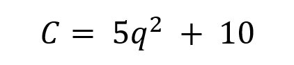
Now, it looks somewhat simple!
Intuitively, you can make out that the cost of production(C) increases as production level(q) increases. Well, let’s plot the curve and try to find some underlying relationships that pass our eye.

Marginal Cost
Looking at the above graph, you can make out that as q increases, C increases. But interestingly, as you might have noticed, the rate of increase in C w.r.t. q increases as q increases. Intuitively, it means that as you increase your production level, the cost of producing the following product will be higher than when your q was low.
‘The more q you want to produce, the more is its cost.’
Mathematically, it means that —

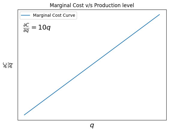
This rate of change in the Cost w.r.t to q is known as the Marginal Cost. Intuitively, it describes the increase in the cost to produce an extra good when you are already producing at a level q.

This is one of the reasons firms cannot produce an indefinite amount of goods in hopes of increasing profits as after a certain level of production, the cost of producing the goods will be higher than what they are sold for.
Average Cost
The average cost can be defined as —
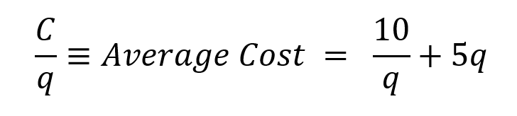
Plotting this function we get —
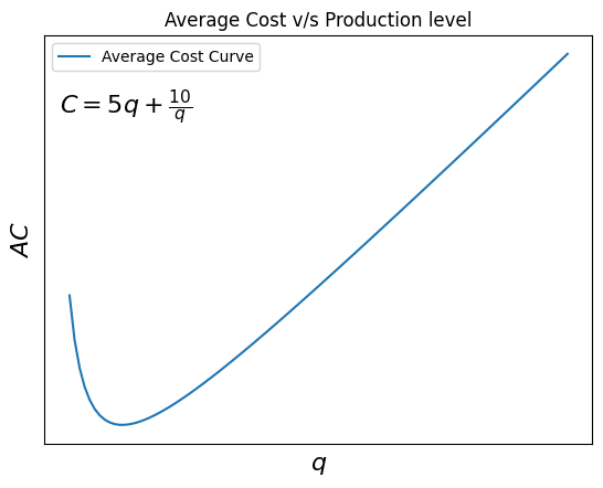
Looking at the plot, we notice something interesting: the AC first decreases and then increases. Well, what does it mean?
Remember, we assumed k to be constant(fixed). Therefore, the first few products sold pay off your fixed costs (k). Hence, your cost of production decreases rapidly, but then the variable costs (wages) start increasing, and therefore, the cost of production starts to increase.
Long Term
Now, coming to the long-term production considerations, we previously assumed capital(k) to be constant for short-term production, but for long-term production, it is continuously variable.
In the long-term, you always have the possibility of increasing your factories, machinery equipment, etc.
Therefore, coming to our Cost Function(C) —
 |
|---|
| Long-Term Cost function |
where,
L = no. of laborers.
k = Capital invested in factories, machinery equipments, etc.
w = Wage rate for the laborers (L)
r = Rental rate
Let us assume,
w = $5
r = $10
Using the above assumptions, we get —
 |
|---|
| Long Run Cost function — ‘Isocost.’ |
Therefore, as discussed earlier, it depends on both L and k.
The long-run cost function is also known as the Isocost of the firm. You can think of it as the budget constraint for the firm.
Marginal Rate of Technical Substitution
As discussed earlier, MRTS is the slope of the Isoquant (q). Mathematically, we can relate it to the Isocost as —
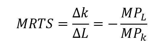

I’ve deliberately skipped the math here, so you can try it out yourself and realize this relationship.
Optimal Choice
As we already know our production function as —

Therefore, plotting the Isocost as well as the production function —

We define Point P1 as the Optimal Choice since it has the highest q value and satisfies the Isocost(C) i.e. we are getting maximum production for our budget constraint. Point P1 is also the tangency point for function q with C.
Shocking the Isocost
What happens if we ‘shock’ our ‘budget constraint’ — Isocost. And more importantly, what happens to our optimal choice of inputs (L and k)??
To keep matters simple, I will only consider the case when w increases, as other cases can also be found via the same way.
Case: Wages increase (w increases)
Imagine you were a bad(evil) boss, and now your overworked workers are staging a protest for a raise. Well, you have no other choice other than to raise the wage rate (w) :(
So, what happens now to your production levels? Will you still be as profitable as earlier using the same budget (cost) you earlier operated with? The answer is a simple no. Therefore, to maximize your profits in this situation, you return to your cost functions and try to salvage what you can get.
Graphically, what it means is —

In the above plot, the dashed lines denote the new Cost Curve (Red) and Production function (Green). As you can see, the new optimal combination of L and k is point P2, and its corresponding q value of sqrt(25) is less than the original q value of sqrt(50).
Therefore, you end up with a lower production level and, hence, less profit when your wage rate is increased. Intuitive right? :)
Long Run Expansion Path
Now, as we are approaching the end of this article, let’s step back and look at the bigger picture of what we have done till now. First, we found the cost function of a firm in both the short and long run. Then, using the long-run Isocosts, we were able to find the optimal combination of L and k the firm should employ to get the maximum output q as well as satisfy the cost of production C.
Now imagine this: Is your q going to remain the same in the future?? Of course not. You, as a business owner, will do anything to increase your production levels and sell more stuff. Now we understand from the above topics that if q increases, C will increase (both in the long-term and short-term), and there is no way around it. Hence, that’s the only ‘path’ you’ll have to take if you are to increase your production level. This ‘path’ is called the Long-Run Expansion Path.
It describes how Cost increases when you want to increase production in the long run.
To visualize this ‘path,’ take a look at the below-given plots.
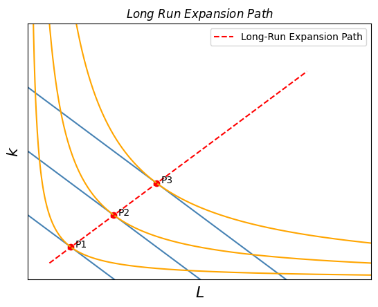
Initially, the optimal choice was point P1, then you increase your Production level (q), simultaneously increasing your Cost of Production as well, and the new optimal choices are points P2 and P3. During your progress from P1 to P2 and P3, the red-dashed line marks your progress and hence is your Long-Run Expansion Path.
I hope you are clear about this.
Sunk Costs
This will be the final topic of this article :)
This is an interesting idea as well, which might not be related completely to any of the above discussions but has an overarching significance in everyone’s lives. And believe me, it does.
In layman’s terms, Sunk Costs can be defined as the Costs that are incurred and cannot be revoked. For e.g. Your insurance payments, college tuition etc.
I hope you get the basic idea.
But in psychological terms, Sunk Costs can paint a very different picture. To get started, imagine you purchased a ticket for a concert night. But the night before the concert, you realize you don’t want to go anymore. Well, what do you do? You find someone who is willing to go, and you try to sell yours to him. Now the big question is, how much will you charge him? Will it be more than what you paid or less, or maybe the same?
Charging more is rarely the case, as the opposite party already senses your desperation to sell the ticket before time runs out. Hence, you end up selling your ticket at a price less than what you paid for earlier. Hence, a loss. If you were an accountant, how would you describe this loss??
Now, let’s move away from money and come to real-life decisions. Imagine you are watching a movie. Halfway through the movie, you realize it’s not what you were looking for, and therefore, you don’t like it. But believe it or not, more often than not, people end up watching the same movie grudgingly, even though they don’t like it. The reason people give themselves is that since they already invested so much time in watching till halfway, might as well watch the other half.
This cognitively biased thinking is known as the Sunk Cost Fallacy, where one continues pursuing his endeavor even after realizing it is a mistake.
More on Sunk Cost Fallacy (link)
Biased thinking like this can lead to much distress in life, especially in investments, relationships, jobs-related decisions.
Conclusion
The above blog covered the basic ideas of Production Costs, Short-term and Long-term considerations. Ultimately, it dived into Optimal Choices and their effect on the input parameters while ending with an introduction to Long-Run Expansion Paths and Sunk Costs.
I believe that this level of base knowledge is enough for us to dive into the world of ‘Perfect Competition’, and its entailing theories and conclusions.
Can’t wait to start that… :)
Thank you again for reading, and goodbye :)